|
Fast Track (US)
|
Researchers, Institutions, Governments, ... have all experienced, Fast-Track Clinical Trials where no study has ever been done to test its safety.
Clinical Data: Game Change 2022 New Players and New Rules
- Researchers using big data to predict the risk of disease and improve patient treatment at Seven Oaks Chronic Disease Innovation Centre Inc
- Biostatistician or an outside consultant review.,, Seek to proactively manage any potential conflicts of interests. International Committee of Medical Journal Editors (ICMJE) http://www.icmje.org/
- 12:04
From the Inform Consent Action Network and the FDA has admitted that their regulatory committee for the COVID vaccines the people on there are basically all have conflicts of interest and ties to pharmaceutical industries but they said they're not going to do anything about it they've refused to and and going back to the medical martial law ... James Corbett on Medical Martial Law, Solutions and Agorism www.youtube.com/watch?v=U1v9DMCW3MU
|
which opened the doors for other companies to also display their theses.
CTV News London at Six for Sunday, January 30, 2022 (17:14 min:sec. into video) https://london.ctvnews.ca/video?clipId=2366634&binId=1.1137524&playlistPageNum=1 |
|
Read More
COVIDWISE - W.L.COLLINS Project Portfolio (weebly.com) https://wlcollins.weebly.com/covidwise.html |
|
VAERS data released Friday by the CDC included a total of 778,685 reports of adverse events from all age groups following COVID vaccines, including 16,310 deaths and 111,921 serious injuries between Dec. 14, 2020 and Oct. 1, 2021.
- Reports of Serious Injuries After COVID Vaccines Near 112,000, as Pfizer Asks FDA to Green Light Shots for Kids 5 to 11 Reports of Serious Injuries After COVID Vaccines Near 112,000, as Pfizer Asks FDA to Green Light Shots for Kids 5 to 11 • Children's Health Defense (childrenshealthdefense.org)
- The Defender is experiencing censorship on many social channels. Be sure to stay in touch with the news that matters by subscribing to our top news of the day. It's free. https://childrenshealthdefense.org/
|
Fact vs. fake - why don’t we trust science any more? | DW Documentary www.youtube.com/watch?v=frCIYEyURV0
06:50 when you see a flourishing of new studies emerge in any particular area, a little bit ironically it creates the appearance of being dedicated to pursuing the truth but it takes me directly back to the case of big tobacco. YouTube banned this video: Alt.: https://communityrights.us/2021/05/11/fact-vs-fake-why-dont-we-trust-science-anymore-dw-documentary/
Why were all the Bees dying? As soon as pesticides were suspected there was a dramatic rise in the number of public and private studies focusing on alternative explanations. The veterinary authorities were confused, the more studies there were the less beekeepers could make sense of it all. Fact vs. fake - why don’t we trust science any more? | DW Documentary www.youtube.com/watch?v=frCIYEyURV0 Covid Vaccines Bloody Travesty: From Shots to Clots By Dr. Joel S. Hirschhorn Global Research September 23, 2021
|
Chapter 2: Escharotics: 500 Years of Suppression
Centuries before Mesmer, Paracelsus understood and employed the principles of suggestion; centuries before Freud, he understood mind/body connection; centuries before Antonio Meucci 5 or R. Raymond Rife, 6,7 he utilized electromagnetic therapy; he discovered hydrogen, nitrogen; coined the term "alcohol" (from the Arabic) 8, and identified zinc. He composed his own pharmacopeia and achieved clinical success that few physicians today can match -- all at a time when medical specialization, as we know it, was non-existent. There are hundreds of botanical extracts, the knowledge of which come to us from indigenous sources worldwide, which have shown to have anti-cancer properties. Dr. Jonathan Hartwell (23), one of the founders of the National Cancer Institute, spent most of his adult life categorizing them, leaving behind a reference that would become a classic in the field of phytopharmacology and ethnobotany. http://meditopia.org/chap2.htm
GAME
Unless you agree to their terms and conditions, you Can't participate. 
|
Perishable Publications
Many, if not most, published research papers have titles that defy comprehension. They use specialized jargon, complex words
and opaque phrases like "nonlinear dynamics." Sometimes they don't, and yet they are still hard to figure out. Here's a
title of a published research study: "Stimuli Eliciting Sexual Behavior." In this case, the specific topic was the sexual
behavior of turkeys, in which a pair of researchers at Pennsylvania State University in the early 1960s wanted to know just
how minimal turkey stimuli might be to still do the job. So they created a mock female bird and progressively removed
parts of the model, assessing when a male turkey lost interest. Finally, they got to just a stick-mounted head and neck,
which the male turkey found just as appealing a mate as a whole bird.
|
|
Courses:combined MD-PhD program, PhD is a degree in clinical research and performing clinical trials
GCP
Canada:
Notice – Release of ICH E6(R2): Good Clinical Practice https://www.canada.ca/en/health-canada/services/drugs-health-products/drug-products/applications-submissions/guidance-documents/international-conference-harmonisation/efficacy/good-clinical-practice-consolidated-guideline-topic.html Clinical Trials: A Practical Approach By Stuart J. Pocock
General Guidelines for Methodologies on Research and Evaluation of Traditional Medicine https://apps.who.int/iris/bitstream/handle/10665/66783/WHO_EDM_TRM_2000.1.pdf You think writing is communicating your ideas to your readers. It's not. It's about changing their ideas/thoughts Source:https://www.youtube.com/watch?v=vtIzMaLkCaM
|
Resources:
The CanLII.org website provides access to court judgments from all Canadian courts, including the Supreme Court of Canada, federal courts, and decisions from many tribunals nationally.
ICH Official web site : ICHhttps://www.ich.org
ICH harmonisation for better health structure and content of clinical study... |
Past Case Examples
Mitigate the potential for bias in analysis of data by involving, for example, an independent biostatistician or an outside consultant review. Seek to proactively manage any potential conflicts of interests.
International Committee of Medical Journal Editors (ICMJE) http://www.icmje.org/
The ICMJE is a small group of general medical journal editors and representatives of selected related organizations working together to improve the quality of medical science and its reporting.
International Committee of Medical Journal Editors (ICMJE) http://www.icmje.org/
The ICMJE is a small group of general medical journal editors and representatives of selected related organizations working together to improve the quality of medical science and its reporting.
Big Pharma - How much power do drug companies have? 2021
www.youtube.com/watch?v=-z_W3yRA9I8&t=37s41:14
the FDA now is on the payroll of the pharmaceutical industry they pay user fees to the part of the FDA that evaluates new drugs for approval so this makes this part of the FDA dependent on the companies that they are supposedly regulating, the drug companies love it because it makes the part of the FDA that evaluates their drugs extremely friendly since they support it. It is a blatant conflict of interest this ought to be well-funded and there ought to be no conflicts of interest [
https://www.cbc.ca/news/canada/thunder-bay/aboriginal-nutritional-experiments-had-ottawa-s-approval-1.1404390
Paragraph. ここをクリックして編集する.
Aboriginal nutritional experiments had Ottawa's approval
Recent research by Canadian food historian Ian Mosby revealed that at least 1,300 aboriginal people — most of them children — were used as test subjects in the 1940s and '50s by researchers probing the effectiveness of vitamin supplements.
Recent research by Canadian food historian Ian Mosby revealed that at least 1,300 aboriginal people — most of them children — were used as test subjects in the 1940s and '50s by researchers probing the effectiveness of vitamin supplements.
Psychotherapy & Older AdultsResource Guide
https://www.apa.org/pi/aging/resources/guides/psychotherapy
physiology and nutrition, Fetal physiology and nutrition. focused around understanding how nutrition impacts fetal physiology and development. We're specifically interested in
pregnancy conditions that the mother may have that may alter normal fetal development. This may include cases when
the mother's placenta doesn't fully develop, or cases when the mother has gestational diabetes or other pregnancy conditions
that impacts nutrient supply to the fetus. Research is relevant to women's health, the study of pregnancy, nutrition of the mother during pregnancy and how that impacts the baby in later life, disease risk for that baby, or early perinatal outcomes for the baby as well.
TOOLS
Best survey tools - at a glance SurveyMonkey, Typeform, JotForm AskNicely Formstack Surveygizmo Google Forms
Extensive coverage from early-stage drugs through approvalhttps://www.drugbank.com
DrugBank includes summaries for over 3,000 clinical drugs, and 7,500 pre-clinical drugs. Each drug is associated with more than 200 different types of information including detailed pharmacology descriptions, chemical structures, chemical properties, drug-protein relationships, and many clinically relevant datasets including adverse effects, indications, and drug-drug interactions.
Our extensive datasets and coverage support diverse use cases relevant to drug discovery: business intelligence research, comparing potential candidates to existing drugs, identifying potential targets, toxicology modelling, and training machine learning models.
|
Snowball Sampling: Definition, Advantages and Disdvantages ...
Conducted an online survey using snowball sampling techniques. Snowball sampling consists of two steps:
Spielberger’s State Trait Anxiety Inventory STAI The STAI, itself, assesses anxiety but also can be used to make a discrimination when wondering whether a patient is experiencing anxiety or depression. This inventory is used in research projects. Various journal articles have used the STAI in conducting research and comparing different ethnic groups, age groups, etc. ANOVA Factorial Experiment Analyzed by Hand Completing an ANOVA table How to Write the Results for an ANOVA Examples of Experimental Designs Experimental Design: Variables, Groups, and Controls Three-level full factorial designs Documentary analysis
Documentary analysis is a type of qualitative research in which documents are reviewed by the analyst to assess an appraisal theme. Dissecting documents involves coding content into subjects like how focus group or interview transcripts are investigated. A rubric can likewise be utilized to review or score an document. The three essential sorts of documents are...More at Wikipedia |
Stomp On Step 1
Null Hypothesis, p-Value, Statistical Significance, Type 1 Error and Type 2 Error SKIP AHEAD: 0:39 – Null Hypothesis Definition 1:42 – Alternative Hypothesis Definition 3:12 – Type 1 Error (Type I Error) 4:16 – Type 2 Error (Type II Error) 4:43 – Power and beta 6:33 – p-Value 8:... CC Is Your Evidence Biased because the algorithm assigned people to high-risk categories on the basis of costs, those biases were passed on in its results: black people had to be sicker than white people before being referred for additional help. Only 17.7% of patients that the algorithm assigned to receive extra care were black. The researchers calculate that the proportion would be 46.5% if the algorithm were unbiased. www.nature.com/articles/d41586-019-03228-6 Finding fixes for bias in algorithms — in health care and beyond — is not straightforward, Obermeyer says. “Those solutions are easy in a software engineering sense: you just rerun the algorithm with another variable,” he says. “But the hard part is: what is that other variable? How do you work around the bias and injustice that is inherent in that society?”
|
It's not that simple
|
56:47 a forest plot
Joe Rogan Experience #1393 - James Wilks & Chris Kresser - The Game Changers Debate https://www.youtube.com/watch?v=s0zgNY_kqlI Meat and poultry, a good source of B12?
|

|
Financial conflicts of interest
The federal government requires that institutions establish and administer a financial conflict of interest disclosure policy to promote objectivity and research.
A conflict of interest means that you, as the investigator have a financial incentive or the appearance of potential financial gain from the findings or outcomes of the research. Think for a moment about whether these situations might influence your study.
reporting of research are disclosed and managed. The government has defined minimum disclosure thresholds, but your individual institutions may adopt policies that are more rigorous.
Disclosures must be reported annually or more frequently if certain financial activities have occurred. Your own institutional policies will guide you through the correct reporting frequency. As noted, conflicts may arise from others within your direct family unit. Therefore, you must also disclose certain financial interest obtained or held by your spouse or dependent children. It's important that you inquire about your institution's financial conflict of interest policies as well as the process for disclosure.
General areas of concern are paid board positions at corporate institutions that fund research, holding stock equity in corporate institutions that fund research or paid speaking and travel engagements. Conflict of interest training is designed to make you aware and your institution aware of situations and relationships that can possibly influence your research work or might have the appearance of influence. Conflict of interest goes beyond financial gain and also includes relationship such as unfunded or voluntary board positions. Education to support unbiased research and disclosure are the main goals.
Meta-analyses with industry involvement are massively published and report no caveats for antidepressants
by S Ebrahim, S Bance, A Athale, C Malachowski…Journal of clinical …, 2016 - Elsevier
Conclusion
1) There is a massive production of meta-analyses of antidepressants for depression authored by or linked to the industry,
2) and they almost never report any caveats about antidepressants in their abstracts.
3) Our findings add a note of caution for meta-analyses with ties to the manufacturers of the assessed products.
Objectives
To identify the impact of industry involvement in the publication and interpretation of meta-analyses of antidepressant trials in depression.
Study Design and Setting
Using MEDLINE, we identified all meta-analyses evaluating antidepressants for depression published in January 2007–March 2014. We extracted data pertaining to author affiliations, conflicts of interest, and whether the conclusion of the abstract included negative statements on whether the antidepressant (s) were effective or safe.
Results
* We identified 185 eligible meta-analyses.
* Fifty-four meta-analyses (29%) had authors who were employees of the assessed drug manufacturer, and
* 147 (79%) had some industry link (sponsorship or authors who were industry employees and/or had conflicts of interest).
* Only 58 meta-analyses (31%) had negative statements in the concluding statement of the abstract. Meta-analyses including an author who were employees of the manufacturer of the assessed drug were 22-fold less likely to have negative statements about the drug than other meta-analyses [1/54 (2%) vs. 57/131 (44%); P < 0.001].
The federal government requires that institutions establish and administer a financial conflict of interest disclosure policy to promote objectivity and research.
A conflict of interest means that you, as the investigator have a financial incentive or the appearance of potential financial gain from the findings or outcomes of the research. Think for a moment about whether these situations might influence your study.
- Your spouse is employed by the company whose drug you are studying.
- Or you have an ownership share of a pharmaceutical company whose drug you were studying.
reporting of research are disclosed and managed. The government has defined minimum disclosure thresholds, but your individual institutions may adopt policies that are more rigorous.
Disclosures must be reported annually or more frequently if certain financial activities have occurred. Your own institutional policies will guide you through the correct reporting frequency. As noted, conflicts may arise from others within your direct family unit. Therefore, you must also disclose certain financial interest obtained or held by your spouse or dependent children. It's important that you inquire about your institution's financial conflict of interest policies as well as the process for disclosure.
General areas of concern are paid board positions at corporate institutions that fund research, holding stock equity in corporate institutions that fund research or paid speaking and travel engagements. Conflict of interest training is designed to make you aware and your institution aware of situations and relationships that can possibly influence your research work or might have the appearance of influence. Conflict of interest goes beyond financial gain and also includes relationship such as unfunded or voluntary board positions. Education to support unbiased research and disclosure are the main goals.
Meta-analyses with industry involvement are massively published and report no caveats for antidepressants
by S Ebrahim, S Bance, A Athale, C Malachowski…Journal of clinical …, 2016 - Elsevier
Conclusion
1) There is a massive production of meta-analyses of antidepressants for depression authored by or linked to the industry,
2) and they almost never report any caveats about antidepressants in their abstracts.
3) Our findings add a note of caution for meta-analyses with ties to the manufacturers of the assessed products.
Objectives
To identify the impact of industry involvement in the publication and interpretation of meta-analyses of antidepressant trials in depression.
Study Design and Setting
Using MEDLINE, we identified all meta-analyses evaluating antidepressants for depression published in January 2007–March 2014. We extracted data pertaining to author affiliations, conflicts of interest, and whether the conclusion of the abstract included negative statements on whether the antidepressant (s) were effective or safe.
Results
* We identified 185 eligible meta-analyses.
* Fifty-four meta-analyses (29%) had authors who were employees of the assessed drug manufacturer, and
* 147 (79%) had some industry link (sponsorship or authors who were industry employees and/or had conflicts of interest).
* Only 58 meta-analyses (31%) had negative statements in the concluding statement of the abstract. Meta-analyses including an author who were employees of the manufacturer of the assessed drug were 22-fold less likely to have negative statements about the drug than other meta-analyses [1/54 (2%) vs. 57/131 (44%); P < 0.001].
Researcher Management and Leadership Training: University of Colorado Anne M. Libby, PhD
This course is for early career researchers and mentors who believe that modern scientific careers require management skills and want to be research leaders. This curriculum gives you skills to effectively implement funded projects, thereby enhancing your career success. Research leaders take on a number of new roles, rights, and responsibilities--as scientific leaders, financial administrators, managers, and mentors. In this course, we explain how to optimize the people, teams.
|
Assess the importance of management and leadership skills, and identify approaches to optimize resources when building a research career.
five practices of exemplary leadership.
1. Model the way - clarify your values, align your actions and words... 2. Inspire a shared vision - that is noble, bold, innovative, and impactful by ... improving human health ...appeal to shared visions/wishes though a common V 3. Challenge the process - optimizing, seeking new ways to grow/improve/change..take the risks, accepting failures along the way 4. Enable others to act - by giving trust and responsibility to others 5. Encourage the heart - convey hope and appreciation for efforts The Five Practices of Exemplary Leadership http://www.leadershipchallenge.com/ The Leadership Challenge, Kouzes and Posner www.youtube.com/watch?v=kUVV3398acQ Kouzes JM, Posner BZ. (2017) The Leadership Challenge: How to Make Extraordinary Things Happen in Organizations, 6th ed., Hoboken, NJ: John Wiley & Sons. "For anyone who wants to improve their leadership, The Leadership Challenge is the perfect book for you." (The association of MBA's, June 2017) https://www.amazon.com/Leadership-Challenge-Sixth-Extraordinary-Organizations/dp/B071V5JHBB |
Identify key financial and administrative responsibilities for researchers, including regulatory compliance, financial reporting, and budgeting.
Compare key responsibilities for mentors and mentees, strategically build mentorship teams, and enhance mentorship using coaching and sponsorship.
|
Alison Lakin - Research Integrity Officer and the Compliance Officer, Alison Lakin.
- As research leader, you will be expected to take action and lead others to take appropriate actions.
- In research, we don't know the answer before we start
- do's and don'ts for successful research,
- build systems and provide training to support the conduct of ethical compliant research that produces quality data,
- Regulatory compliance and ethical compliance, rules provide the floor, not the ceiling. Researchers should view the regulations and the ethics of research as the minimum bar for what is right and good
- For the first tip, reduce the potential for bias. If you knew the answer to the question, then you wouldn't need to study it, right? Remember that the best hypothesis have meaningful information and advanced science no matter what the result. Nevertheless, it's not hard to get very attached to our beliefs, and that can introduce internal bias
- Examples of controls to reduce bias are using blinding in random allocation, so no one knows who is in the experimental condition, or developing your analysis plan up front, not after the fact, to reflect how you want to best show the data to avoid data mining. You can also build your own research management systems to have internal checks and balances. By this, I mean that more than one person should do the experiment or collect the data independently and record the findings independently, so that it's not over-reliant on one person. This also helps with reproducibility. It ensures that inherent bias of how one person is doing things is not unduly impacting the data. If you have the ability to replicate it in other labs or sites, that is, have a collaborator to be the second tester completely outside of your lab, then do that too. This shows that you are doing reproducible science, and it's not something that only you can do to get those results.
- My second tip is follow the protocol. Putting your creative ideas on paper in a way others can follow is a challenge. You have to design your study, then develop a research protocol that reflects what you're actually going to do, and that you plan to follow as a guide in a way that others, not necessarily even in your field, can follow. A protocol is not just a piece of paper that you submit to a compliance committee. Whether you seek approval from a committee that protects human or animal subjects or addresses biosafety or radiation safety, that protocol is your roadmap, and not just a check the box to be able to do research.
- Now, of course, there's an art to successful committee reviews. First remember to consult with your compliance officer for help and guidance. Next, practice what I call the art of "vague specificity." That is, you need to be specific enough that the compliance committees understand your research plan and know what you're trying to do. But have it in inherent flexibility so that you can adapt to and learn from the research as you move forward, so that you're not always amending the protocol every five minutes. That said, please remember that changes significant enough to need a protocol amendment need to be approved by the compliance committees before you actually implement the changes.
- two pro tips for avoiding problems and maintaining good compliance as a researcher.
Tip one, do a feasibility assessment. - that is make sure that you're balancing the Integrity of the science with the art of what is practical because it's not going to help you to get part way through and then realize that you can't do this research in the approved scope of time and resources. Make sure you have the right equipment and you have the skill sets to use it and collaborate when needed. If you're going to collaborate and this is also true for delegation in your own lab then trust but verify any data that you do not control. Your goal is that you're comfortable standing behind all that data that's in this research. - Tip two train and train again. You need to have a business continuity plan. Training more than one person helps. Having good documentation helps. Having training manuals helps. and really do make a difference and help in the quality of the data when you have staff turnover or you have students coming through that move on And remember that if you don't do a task frequently then it's okay to do a refresher, sometimes people need to relearn and to get comfortable doing that task again. As the research leader, you should provide to create an environment where it's okay to ask for help.
- Most journals have clearly specified authorship criteria to it's good to have an objective criteria and go through the process of listing out who actually did what on a paper.. Anyone listed on a manuscript should be able to stand behind the data. So putting people on papers just because it will look good for the next grant submission is not appropriate. People need to take responsibility for the data as well as enjoy the credit so they need to contribute, they need to be comfortable with the data, they need to have reviewed the paper. Follow the International Committee of Medical Journal Editors, ICMJE guidelines, as an objective criteria to determine authorship. Effective research leaders have a written manuscript plan that includes topical scope, target journal, and authorship plans in order of authorship. As part of this plan for authorship, you address this early before writing.
- Data storage and management is critical. You need a robust data management plan for your research, and this is a long term commitment. For example, we've had opportunities to have the US Food and Drug Administration, the FDA, audit research studies that were conducted 20 years ago. So know where data are recorded, be able to produce it on request. It can be challenging, it's a long-term process that can be hard, especially now with the changing technology. Think of computer software and hardware changes. Be thoughtful as to what your long term data storage and your data sharing
strategies are, and build these into your budget at the beginning of the study. Find out from your institution what data storage capacity they're investing in that might help you. - protect clinical data. Clinical data that is data on human subjects and healthcare patients is protected at the highest level from a research perspective. Not only from a research integrity perspective, but also due to privacy requirements, and due to sensitivity around personal health records. Even a simple procedure like a blood draw is more than just a blood draw, with someone's blood, you have a link to a person's genetic code. Use the database that is designed to comply with the US Health Insurance Portability and Accountability Act, also known as HIPAA.
- Tip, manage conflicts of interest. It's important to recognize that we're all conflicted, and in terms of the roles that we have within the lab, within the project, within the institution, whether it's time management, whether it's conflicting priorities, or the big one that is emphasized today, financial conflicts of interests. Conflict of interest is under particular scrutiny with commercial for-profit companies. In my opinion, we need relationships with drug and device companies. They're important in order for us to really move research and scientific developments into the healthcare arena. It's difficult to manage the perception of conflicts of interest with these entities, and so be very thoughtful about when you enter into relationships with drug and device companies. Mitigate the potential for bias in analysis of data by involving, for example, an independent biostatistician or an outside consultant review. Seek to proactively manage any potential conflicts of interests.
The ICMJE is a small group of general medical journal editors and representatives of selected related organizations working together to improve the quality of medical science and its reporting.

Ankylosing spondylitis these people have a gene called HLA-B27
Ankylosing spondylitis - Wikipedia
https://en.wikipedia.org › wiki › Ankylosing_spondylitis Ankylosing spondylitis. Other names. Bekhterev's disease, Bechterew's disease, morbus Bechterew, Bekhterev–Strümpell–Marie disease, Marie's disease, Marie–Strümpell arthritis, Pierre–Marie's disease. A 6th-century skeleton showing fused vertebrae, a sign of severe ankylosing spondylitis. |

Psoriatic patients
Frequencies of HL-A antigens, blood groups (ABO, Rh, MNSs, Kell, Lewis and Duffy), serm groups (Hp, Gc and C3) and red cell enzyme types (PGM1· 6-PGD and AK) were studied in a series of 122 psoriatic patients from northern Sweden. The increased frequency of the HL-A antigens W17 and HL-A13 found in previous investigations was confirmed. An association was found with the MNSs blood groups, Ss heterozygotes being strongly underrepresented among psoriatic patients. The frequencies of the blood type Le (a–b–) in the Lewis system and the A-factor in the ABO-system were found to be increased in proriasis. In the psoriatic patients a significant deficiency of heterozygotes was found in the Hp and C3 serum groups.
|

Metformin - The Case of Exaggerating Both Benefits and Harms
Fat Chance: Fructose 2.0
|
|
In Germany only eight percent of the population have the HLA-B27
Bechterew's disease, rheumatism, spondylitis - arthrosis is something else - important tips for everyday life Welcome to the topic of disease https://www.youtube.com/watch?v=n6Ey3C2AU80 Ankylosing spondylitis has no known specific cause, though genetic factors seem to be involved. In particular, people who have a gene called HLA-B27 are at greatly increased risk of developing ankylosing spondylitis. However, only some people with the gene develop the condition. |
|
EPA Radon Zones (with State Information) HLA-B27 well you have a greater increased risk of developing Ankylosing Spondylitis
The Map of Radon Zones was developed in 1993 to identify areas of the U.S. with the potential for elevated indoor radon levels. The map is intended to help governments and other organizations target risk reduction activities and resources.
There use to be a theory called The Linear-No-Threshold (LNT) theory which states that the dose-effect response is the same per unit dose regardless of the total dose. With all the NUCLEAR DUMPING sites showing up around the Great Lakes (https://www.michiganradio.org/post/were-closer-decision-underground-nuclear-waste-site-near-lake-huron) it's no wonder this theory has been challenged.
Radon
Radon is a chemical element with the symbol Rn and atomic number 86. It is a radioactive, colorless, odorless, tasteless noble gas. It occurs naturally in minute quantities as an intermediate step in the normal radioactive decay chains through which thorium and uranium slowly decay into lead and various other short-lived radioactive elements; radon itself is the immediate decay product of radium.
https://en.wikipedia.org/wiki/Radon
Radium
Radium is a chemical element with the symbol Ra and atomic number 88. It is the sixth element in group 2 of the periodic table, also known as the alkaline earth metals. Pure radium is silvery-white, but it readily reacts with nitrogen on exposure to air, forming a black surface layer of radium ... nitride.https://en.m.wikipedia.org/wiki/Radium
Governments want to make you feel better regarding the fact you live in a nuclear dumping ground. Here are two two articles smoothing over the inevitable fact you are exposed to Radon.
1. Health Effects of High Radon Environments in Central Europe: Another Test for the LNT Hypothesis?
https://www.ncbi.nlm.nih.gov/pubmed/19330110/
2. Radon Treatment Controversy
https://www.ncbi.nlm.nih.gov/pmc/articles/PMC2477672/
3. The Radium Girls: The Dark Story of America’s Shining Women, Kate Moore tells the story of how these dial painters took on the radium companies that made them sick—as they were dying of radium poisoning.
Video: https://www.youtube.com/watch?v=BlgC4hQ8i5E
https://www.youtube.com/watch?v=n6Ey3C2AU80
Source:
https://www.epa.gov/radon/find-information-about-local-radon-zones-and-state-contact-information
To be classified as a radon mineral water, it must have a minimum of 2 nCi/L (74 Bq/L) concentration of radon. Radon baths are typically used for hypertension, rheumatoid arthritis and arteriosclerosis of lower extremities, and inhalation therapy is often administered at speleotherapy centers for conditions such as chronic bronchitis and bronchial asthma. Compared to baths, inhalation radon is absorbed at a faster rate via mucous membrane (Ponikowska et al. 2002).
and “scientific” healing has maimed and killed millions! Ever hear of thalidomide? Vioxx? Tuskegee syphilis experiment? frontal lobotomy? Mercury in vaccines? Forced sterilization? etc ad nauseum….. Science is not better or even good. It just is and you have decided to worship it as your religion.
|
What is beneficence in research?
Beneficence is a concept in research ethics which states that researchers should have the welfare of the research participant as a goal of any clinical trial or other research study. The antonym of this term, maleficence, describes a practice which opposes the welfare of any research participant. en.wikipedia.org › wiki › Beneficence_(ethics) Beneficence (ethics) - Wikipedia Search for: What is beneficence in research? What are the 5 categories of risk identified under the concept of beneficence? The three basic principles are (1) respect for persons, (2) beneficence, and (3) justice. In this context, the principle of beneficence is understood as an abstract norm that includes derivative rules such as "Do no harm," "Balance benefits against risks," and "Maximize possible benefits and minimize possible harms."Jan 2, 2008 plato.stanford.edu › entries › principle-beneficence The Principle of Beneficence in Applied Ethics (Stanford ... Search for: What are the five categories of risk identified under the concept of beneficence? |
|
|
Tuskegee syphilis experiment - Wikipedia
Tuskegee Study of Untreated Syphilis in the Negro Male was a clinical study conducted between 1932 and 1972 by the U.S. Public Health Service. The purpose ... Eunice Rivers Laurie · Peter Buxtun · United States Public Health · Belmont Report People also ask What happened in the Tuskegee syphilis experiment? The Tuskegee Study of Untreated Syphilis in the Negro Male was an infamous and unethical clinical study conducted between 1932 and 1972 by the U.S. Public Health Service. ... Of these men, 399 had latent syphilis and 201 did not have the disease. en.wikipedia.org › wiki › Tuskegee_syphilis_experiment Tuskegee syphilis experiment - Wikipedia Search for: What happened in the Tuskegee syphilis experiment? What was the purpose of the Tuskegee syphilis experiment? In 1932, the Public Health Service, working with the Tuskegee Institute, began a study to record the natural history of syphilis in hopes of justifying treatment programs for blacks. It was called the “Tuskegee Study of Untreated Syphilis in the Negro Male.” www.cdc.gov › tuskegee › timeline Tuskegee Study - Timeline - CDC - NCHHSTP Search for: What was the purpose of the Tuskegee syphilis experiment? Why was the Tuskegee syphilis study unethical? The study became unethical in the 1940s when penicillin became the recommended drug for treatment of syphilis and researchers did not offer it to the subjects. Q. How did revelations about the study change the way we conduct Public Health Research today? www.cdc.gov › tuskegee › faq Tuskegee Study - Frequently Asked Questions - CDC - NCHHSTP Search for: Why was the Tuskegee syphilis study unethical? |
What was the ethical issues of the Tuskegee Syphilis Study?
Evidently, the rights of the research subjects were violated. The Tuskegee Study raised a host of ethical issues such as informed consent, racism, paternalism, unfair subject selection in research, maleficence, truth-telling and justice, among others. www.ajol.info › index.php › article › download AA Ogungbure The Tuskegee Syphilis Study, Some Ethical ... - AJOL Search for: What was the ethical issues of the Tuskegee Syphilis Study? Did the Tuskegee Airmen have syphilis? The now well-celebrated Tuskegee Airmen have received a number of honors after decades of neglect. But for many black Americans Tuskegee also reminds of the experiment done on black men from 1932 until 1972. The U.S. government injected the men with syphilis. They went untreated as human guinea pigs.Apr 9, 2009 www.sun-sentinel.com › news › trending › sfl-mtblog-2009-04-many_a... Tuskegee fame: Airmen and experiment - South Florida Sun-Sentinel Search for: Did the Tuskegee Airmen have syphilis? Where did syphilis originally come from? Columbian theory This theory holds that syphilis was a New World disease brought back by Columbus, Martín Alonso Pinzón, and/or other members of their crews as an unintentional part of the Columbian Exchange. Columbus's first voyages to the Americas occurred three years before the Naples syphilis outbreak of 1495. en.wikipedia.org › wiki › History_of_syphilis History of syphilis - Wikipedia Search for: Where did syphilis originally come from? Why are ethics important in healthcare? Ethical standards may promote the values of cooperation and collaborative work. Finally, ethical standards in medical care promote other important moral and social values such as social responsibility, human rights, patients' welfare, compliance with the law, SMC's regulations, and patients' safety.Mar 10, 2006 citeseerx.ist.psu.edu › viewdoc › download Medical Ethics: What is it? Why is it important? - CiteSeerX Search for: Why are ethics important in healthcare? |
|
|
The way the research question is asked implies the research method. for example:
|
1. "What is the effect of A on B?"
|
"What is the relationship between
C and D?"
|
"What is the prevalence and distribution of various types of E?"
|
"What is the experience of nursing a first born? nature of F?"
|
Introduction and Experimental Design Basics: Comparative Experiments and Basic Statistical Concepts
|
Module 1
Include the first three steps in your Project Report. 1. Define the problem statement and the objectives of the experiment. 2. Identify your response variable(s) a. How will this be measured? 3. Describe your Factors (at least 3) a. What are the levels for each factor? If continuous, what is the range? b. Do you need/have a blocking variable? |
Module 2
Introduction to Design and Analysis of Experiments all of those experiments had only two levels. The factor only had two levels. Reading: Unit 1 Introduction 10 min Video: LectureHistory of DOX Video: LectureThe Basic Principles of DOX Video: LectureFactorial Designs with Several Factors Practice Quiz: Concept Questions 3 questions on experimental design is of comparative experiments and then some basic statistical methods that are used to analyze the data from those types of experiments. All of the experiments had only two levels. The factor only had two levels. Here the factor could have multiple levels, more than two. Random samples and how to summarize data from those samples. Numerical measures: 1. the sample average or sample mean 2. sample variance 3. the standard deviation, Graphical methods: Populations versus samples and parameters of populations like the population mean or population variance and standard deviation ...How to estimate parameters with the sample data. ..................................... How to analyze data from simple comparative experiments using the framework "the hypothesis testing framework" The principle hypothesis testing technique is the two-sample t-test. Variations of the two-sample t-test is the primary analysis engine that is used for looking at data from these simple experiments. Checking Assumptions and what the importance of those assumptions are, and how violations of those assumptions might be some threat to the validity of your experiment. |
Module 3
Simple Comparative Experiments Reading: Unit 2 Introduction 10 min Video: LectureComparative Experiments and Basic Statistical Concepts 10 min Video: LectureThe Hypothesis Testing Framework 14 min Video: LecturePooled t-test and Two-sample t-test Video: LecturePooled t-test and Two-sample t-test, pt 2 Video: LectureHypothesis Testing on Variances Video: LecturePaired t-test Video: LecturePortland Cement Data Example Video: LectureFlorescence Data Example Video: LectureHardness Testing Example Practice Quiz: Concept Questions 3 questions Module 3 on experimental design Here the factor could have multiple levels, more than two. The t-test that we studied before, it just doesn't work. It does a really nice job of comparing the means of two factor levels, but it doesn't really work nicely for more than two factor levels. There's no really easy way to make it work. Of course, there are lots of practical situations where there are either more than two factor levels of interest. |
Module 4
Introduction and Experimental Design Basics Week 4 factor could have multiple levels, more than two. Experiments with a Single Factor - The Analysis of Variance Reading: Unit 3 Introduction: Experiments with a Singe Factor; the Analysis of Variance 10 min Video: LectureAnalysis of Variance (ANOVA) 12 min Video: LectureModels for the Data 10 min . Click to resume Video: LectureANOVA for Plasma Etching Experiment 9 min Video: LecturePost-ANOVA Comparison of Means Video: LectureSample Size Determination Video: LectureExamples of Single-Factor Experiments Video: LectureThe Random Effects Model Video: LectureExample of Random Factor Experiment Video: LecturePlasma Etching Example 5 min Video: LectureFabric Strength Example 2 min Practice Quiz: Concept Questions 4 questions |
Module 5
Randomized Blocks, Latin Squares, and Related Designs Reading: Unit 4 Introduction: Randomized Blocks, Latin Squares, and Related Designs; techniques for handling nuisance factor is experiments LectureThe Blocking Principle LectureExtension of the ANOVA to the RCBD LectureExample LectureResidual Analysis for the Vascular Graft Example LectureThe Latin Square Design LectureVascular Graft Example Practice Quiz: Concept Questions 4 questions |
Typical simple comparative experiment.
|
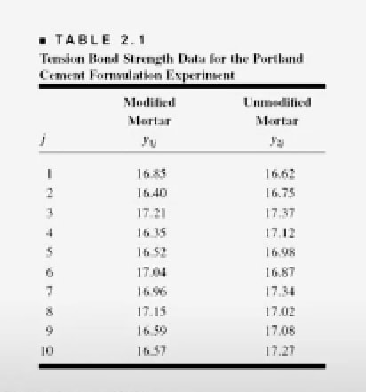
We have a group of engineers who are trying to improve the performance of a product and this product is Portland cement. What they've done is they've taken the original recipe for the mortar and they've modified it by adding polymer latex materials in an effort to reduce the setup time or the drying time of the mortar. This has been very successful.
They've observed a very dramatic change in the drying time. So that part of the experiment is over and now what they're looking at is the tension bond strength as adding this material to the recipe changed the bond strength of the cement. |
|
To test this, they have prepared
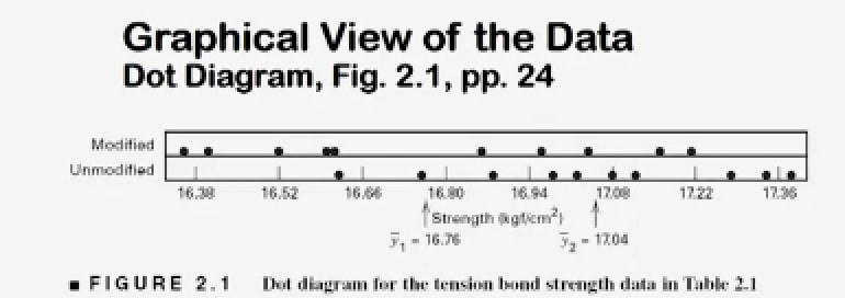
that they've observed in testing. This sample data will be used for the t-test. How do we visualize this data? 1. dot diagram 2. stem-and-leaf plot 3. histogram. 1. Dot Diagram: a scale, either horizontal or vertical, portraying the sampled data as dots along that scale. In this case, the two dot diagrams are stacked on top of each other with the modified mortar dot diagram on top and the unmodified mortar dot diagram on the bottom.
|
|
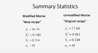
You can see that the calculated the average bond strength for both of these formulations. The tension bond strength, y bar 1 16.76, is the modified mortar, and 17.04 is for the modified mortar.
|
It appears that the average of
the modified mortar is probably a little lower than the average of the unmodified mortar and in fact, the numbers reveal that 16.76 for the modified mortar and 17.04 for the original recipe. |
the spread of the observations is about the same.
That is if you look at the spread here and compare that to the spread here, they're very similar. So you might suspect that the averages or means might have been affected by this change in the recipe, but perhaps not the inherent variability. |
can get a little busy
and not very easy to construct or to interpret for larger samples. |
Dot Diagram
|
Histogram
|
Box Plot (Box whisker plots)
the Z-test
if the sample sizes are large enough, this works okay.
|
T-test
Gosset developed the T-test as the way to specifically answer this question
the 2-sample or the pooled t-test
it measures how unusual the event is.
|
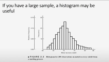
construct a histogram
This histogram is for 200 observations on metal recovery or yield from a smelting process. You can see that the average metal recovery is somewhere around 70 or 71 or 72 percent and that there's a fair amount of variability. It goes all the way from about the low 60s' up to almost 85 percent. But the shape of the distribution is relatively symmetric. |
|
Box Plot construction (spread = whiskers)
|
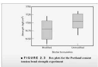
These are the box plots for the Portland cement data that we've looked at earlier.
|
|
|
When you look at these box plots for our two formulations of the mortar, what do you notice?
- in both cases the median, LAN, is in about the middle of the box.
- All right, that tells you that the sample is probably drawn from a symmetric distribution.
- if you look at the length of the boxes, including the whiskers, they're about the same on both of these displays. So that's an indication that the variability in the two populations are probably very similar.
- The other thing that you notice is that the central tendency of the unmodified mortar does appear to be higher than the central tendency of the modified recipe. That's kind of an important issue because if adding this material to the recipe really greatly improved the cure time, this was a victory. But if it has a negative impact on strength, this may affect the usability of the product. So probably what one would want to do after seeing this data is to investigate whether or not there is statistical evidence to support the claim that the main tension bond strength in these two recipes is the same and that's the problem that we'll start to address next.
The Statistical Hypothesis Testing Framework
two-sample t-test procedure.
|
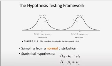
Here's a picture that illustrate visually, the hypothesis testing framework.
The two diagrams are probability distributions. And the probability distribution on the left represents = the population of measurements from factor level 1 or treatment 1. And on the right = the population of measurements from factor level 2 or treatment level 2. |
|
|
In our problem,
each of these represent a different formulation of the Portland cement mortar. Assume that these populations are normal random variables. They're normally distributed observations. The mean of sample of population 1 is mu1 and the variance of that distribution is sigma 1 square. And on the right, those observations are also normally distributed,and that is a normal distribution with mean mu2 and variance sigma 2 square. |
So this is the sampling situation.
This is the situation that we assume exist that we're studying. The key thing here is that we're sampling from a normal distribution. What we want to investigate is the claim that the means of these two populations are the same. |
How we structure that
is in terms of a pair of statistical hypotheses. H-naught is called the null hypothesis. And that's the statement that says the two means are indeed equal. So H-naught, mu1 equal to mu2 is the null hypothesis, and H1 is the alternative hypothesis and that's the other state of nature. And in this case, it would be that the two means are not the same. |
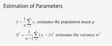
How do we estimate these parameters?
We have a mean mu in each population and we have a variance sigma square in each population. The way we do this is by using the sample average y-bar to estimate the population mean. |
the way you calculate the sample average
is easy. You simply add all the observations in the sample together and divide by the sample size n. |
calculate the sample variance
One simply computes the differences between each observation in the sample and the sample average y-bar squares those differences add them up. And then we divide that sum by n- 1 and that estimates the variance sigma square. These are straightforward calculations. |
Here's the results
|
|
|
|
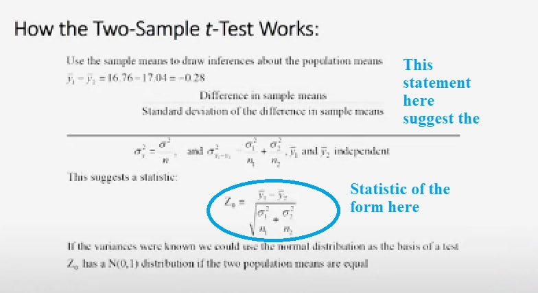
So how does the two-sample t-test work?
it uses the sample means to actually draw conclusions or draw inferences about the population means. And specifically, it uses the difference in those two means. Y-bar 1 minus y-bar 2. |
|
Well, if we plug in the sample data here, the difference in the sample averages y-bar 1- ybar 2 turns out to be -0.28. So that's the difference in the sample means.
The way the t-test works is we then divide that difference in the sample means by the standard deviation of the difference in sample means.
So this ratio becomes a measure of how different the sample means are in standard deviation units. That's how this works.
Well, we know that the standard deviation of an average sigma square of y-bar is sigma square the variance of an individual observation divided by n, the sample size. That's that's basically Statistics that we've probably seen before.The standard deviation of the difference in averages, sigma square of y-bar 1-
y-bar 2 is the sum of those sample variances, sigma 1 square over n1 plus sigma 2 square over n2, as long as the two averages y-bar 1 and y-bar 2 are independent.
- And I think we can comfortably assume independence here, because these are two completely different samples that were generated at different times.
- They're random samples and the treatments were applied essentially in random sequence.
- So independence is probably a very reasonable assumption here.
So this statement here suggest a statistic of the form that you see here.
This ratio is z-naught is y-bar 1- y-bar 2, that's the difference in sample averages. And the denominator of that ratio is the square root of sigma 1 square over n1 + sigma 2 square over n2. That is the standard deviation of the difference in sample means.
Now, how do we use this information?
Well, if the variances were actually known, if we actually knew sigma 1 square and sigma 2 square, it turns out that this ratio z0 follows a normal distribution.
And in fact, if the two means are equal, if mu1 is equal to mu2, this ratio would have a standard normal distribution. That is a normal distribution with mean 0 and variance 1. And we could use that as the basis of a statistical test. And we're going to see how that works, right now.
|
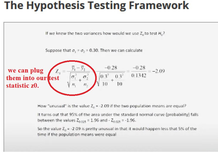
Here's the way it works.
Now, we don't know the variances or standard deviations but let's assume we do. Let's just make up a number. Let's let sigma 1 and sigma 2 both be equal to 0.3 just for purposes of illustration, okay? Soon as we know those two numbers, we can plug them into our test statistic z0. It's what we call z-naught at test statistic. Okay, we plug in the numbers, we do the arithmetic, and that value of z-naught turns out to be -2.09. Okay, now here's how we use that information. Now, we don't know the variances or standard deviations but let's assume we do. Let's just make up a number. |
|
Let's let sigma 1 and sigma 2 both be equal to 0.3 just for
purposes of illustration, okay? Soon as we know those two numbers, we can plug them into our test statistic z0. It's what we call z-naught at test statistic. Okay, we plug in the numbers, we do the arithmetic, and that value of z-naught turns out to be -2.09. |
Okay, now here's how we use that information.
How unusual is this value of z-naught = -2.09 if the two population means are really equal? Well, remember z-naught, if the means are equal, has a normal 01 distribution. Well, in a normal 01 distribution, it turns out that 95% of the probability or area under that normal curve falls between the values 1.96 and -1.96. 1.96 is called the upper 2 1/2 percent point of the normal distributions denoted z sub 0.025, and -1.96 is the lower 0.025 percentage point of the standard normal. |
So if the means are equal, 95% of the time, you would expect to see and observe value of z-naught that's in that interval, -1.96 up to +1.96.
So what about this value that we just calculated, -2.09? That's pretty unusual, isn't it, if the means are equal. This is a value that would only occur less than 5% of the time if the population means were equal. So this is a fairly strong indication that those means are not equal. You can find these z values from any standard normal table. |
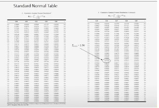
Z Score Table.
|
This is a standard normal cumulative distribution table, and it plots values of z from 0 up to about 3.99.
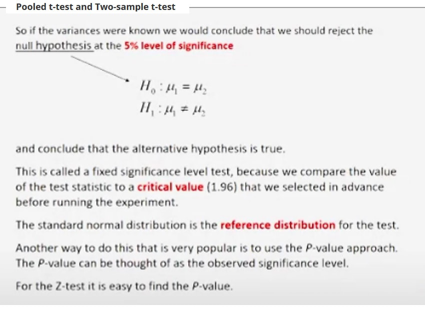
Most standard normal tables are organized like this one. They only give you areas to the left of positive z scores or positive z values. Now, that isn't really much of a problem, because the normal distribution is symmetric and so areas to the left of a negative z are the same as the areas to the right of a positive z. So it's very easy to actually use these tables to show you how I got that value of 1.96. Simply look at the table and scan the table until you find 1.96. Well, here's 1.96 right there. The 1.9 row and the .06 column. And if you look at the entry in the body of the table in 0.975, that is the probability or area to the left of 1.96 on the standard normal curve. So the upper alpha percentage point z of 0.025 would be 1- that. So that's the upper 2 1/2 percent point of the standard normal distribution. And you can use the normal table to calculate these probabilities, or to find these probabilities, or z score values very easily. So if the variances were known, what would we conclude? We would conclude that we should reject this null hypothesis, and a statistician would say we would reject this hypothesis, this null hypothesis at the 5% level of significance. Because the calculated value of -2.09 is outside the + or -1.96 range that corresponds to 5% significance. This is called a fixed significance level test. Because we compared the value of the test statistic to a critical value, in this case 1.96, that we typically select in advance before we run the experiment. And the standard normal distribution is called the reference distribution for this test. Now, there's another way to do this. It's very popular and it's called the P-value approach. The P-value is basically the observed actual significance level. And for the Z-test, it's really easy to find the P-value. And I'll show you how to do that next time. |
P-value approach.
|
|
|
Okay.our last class,
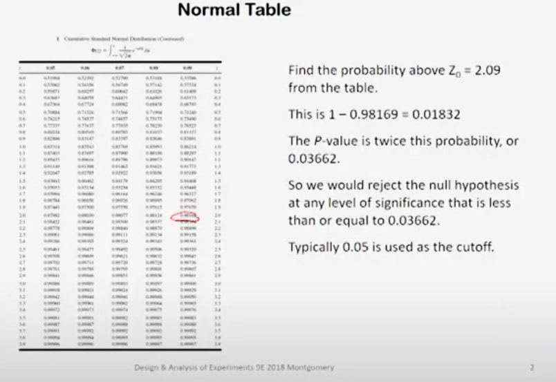
we talked about testing these hypotheses about our Portland cement mortar, and we concluded that we should reject this null hypothesis at the five percent level of significance. So in other words, we've have pretty strong evidence here that the alternative hypothesis is true. We used a procedure that I call up a fixed significance level test because we suggested or proposed a critical value of 1.96 that gives me a five percent chance of being wrong if I conclude that the means are different, if the value of the test statistic lies outside this range of minus 1.96 up to plus 1.96. This fixed significance level approaches is very common, very widely used. But there's another approach that is also very popular and it's actually become popular because of using computer software to do these tests. That's called the P-value approach and for a Z-test, its very easy to find the P-value. Here's how you do it. Here is your standard normal table again that I showed you last time. We want to find the probability above or the probability that the standard normal variable is greater than 2.09. Now, if you think about this for a moment, you say, "Wait a minute. Didn't we calculate the Z_0 was equal to minus 2.09?" Yes, we did, but our table only contains positive values of Z. So we need to take the absolute value of that, and enter the table and find the probability that is above and is greater than positive 2.09. So we go into the table and we look for a value that's greater than 2.09. There it is, 0.98169. All right, the 98169. That is the area to the left of 2.09. We need the area to the right of 2.09, and so that is 0.01832. Just subtract 0.98169 from one. So the P-value will be twice this probability. Why twice. Well, it's a two-sided test, and so you want half of the risk of being wrong to be on one side of zero and the other half to be on the other. So the P-value for this test is actually twice this computed probability. Well, twice that probability is 0.03662. So we would reject this null hypothesis at any level of significance that is less than 0.03662. Typically, in most science and engineering applications, 0.05 is used as the cut-off. Although frankly, there's nothing magic about 0.05, you could use 0.01 or 0.02 or really any value you want. This value of 0.05 is basically a risk measure. It's the risk of you being wrong when you conclude that the means are different. Depending on the consequences of that, you may choose larger or smaller values of the cut-off depending on the context of the problem. I believe that in the early stages of experimental work, where you're really doing a lot of discovery and you're trying to find out which factors in a system might be important, you could be a lot more liberal with your choice of a cut-off. You could use 0.1 or you could use even 0.15 in some cases. But the problem is if you wrongly conclude that a factor isn't important early on in research work, quite frequently what happens is that factor is then ignored and we don't pay any attention to it for the rest of the work. If the factor really turns out to be important, that could have negative consequences on our work. So making some, what we call type I errors, that is concluding that factors are important when they really aren't in the early stages of research work, that's typically not that big a problem because ultimately we will figure out that factors are important or not, but you don't want to throw away all useful one too early. |
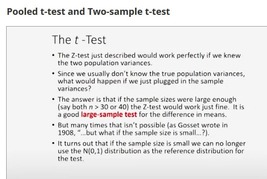
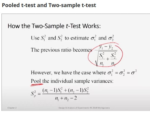
Now, the Z-test, which we've just described works great if you know what the two population variances are, but we don't.
If we knew them, we'd be in great shape. But what if you just plugged in the sample variances instead? Instead of Sigma_1 square in your Z-statistic, plug in s_1 square, and instead of Sigma_2 square in your Z-statistic, plug in s_2 square. Well, if the sample sizes are large enough, this works okay. By large, I mean that the sample sizes for both of your samples would have to be at least about 30, some people say 40. In other words, the Z-test is a very good large-sample test for the difference in means. So if the sample size is big, whether you know the variances or not, is not as big a deal. But many times that isn't possible because your sample size is small. In fact, Gosset actually wrote a paper on the probable error of a mean. said, "But what if the sample size is small?" Well, it turns out if the sample size is small, you can't use this normal 0,1 distribution as your reference distribution anymore. So let's talk about using s_1 square and s_2 square to estimate the two variances. Well, now your previous ratio, your Z-statistic now changes. it looks like this. Instead of Sigmas, it's got Ss. But now remember, we're talking about the case where these variances are assumed to be equal. So let's combine or pool the individual sample variances to get a single number. What you see down at the bottom of this slide is the pooled estimate of variance S square_P. The way this is done it's a weighted average. We simply combine the two sample variances, s_1 squared and s_2 squared, in proportion to the sample sizes. So this is a pooled estimate of variance and when we plug that in, then we get the test statistic for the two-sample T-test, or some people call this the pooled t-test because we've used this pooled estimator variance. |
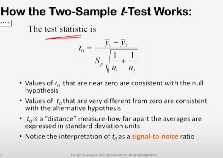
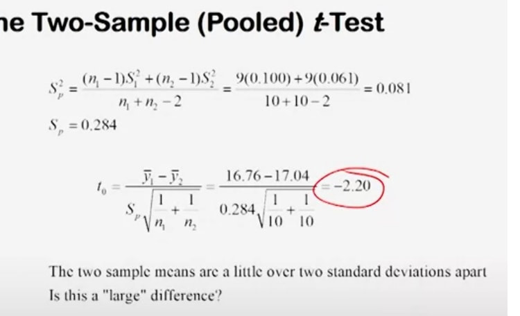
It works a lot like the Z-test that we described earlier. Values of t_0 that are close to zero are consistent with the null hypothesis. Values of t_0 that are very different from zero are consistent with the alternative. So t_0 is a distance measure, just like the Z-statistic was. It measures how far apart the averages are in standard deviation units. You can interpret t_0 as a signal-to-noise ratio. The numerator is a signal that's being generated by your sample data from your experiment, and this thing down in the bottom is a measure of variability, scatter or spread or noise. So when you think of t_0 as a signal-to-noise ratio. So here's how we perform the two-sample or pooled t-test for the Portland cement problem. First of all, we have to calculate S square of P. That's straightforward and we get a calculated value of 0.081 and the square root of that is 0.284. So now, we substitute that into our test statistic t_0, and we get minus 2.20 as the computed value of our test statistic. So the two sample means are a little bit more than two standard deviations apart. Is this a large difference? In other words, how unusual is this value if the means are really equal? |
|
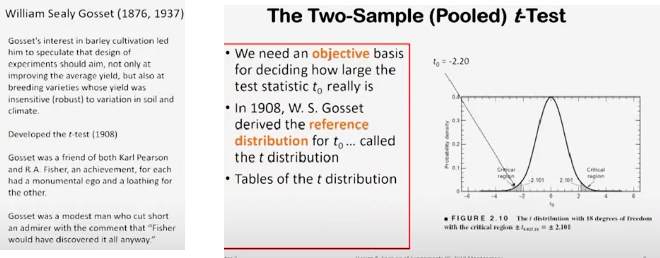
Well, that's the question of course, Gosset answered. Gosset developed the T-test as the way to specifically answer this question.
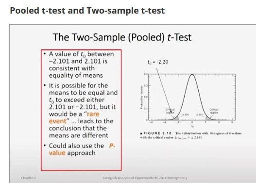
Here's a picture of a t-distribution. The t-distribution looks a lot like the normal distribution, it's symmetric around zero. It has a little bit more spread in the tails than the normal distribution. In this case, the spread in the t-distribution is controlled by something called the number of degrees of freedom on T. The number of degrees of freedom on T here would be the sum of the two sample sizes, N_1 plus N_2 minus 2. So it'd be 18. |
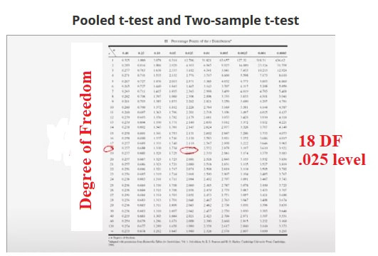
We can use a table of the t-distribution to find, let's say, the two-and-a-half percent point of T with 18 degrees of freedom, and that value turns out to be 2.101.
So minus 2.101 and plus 2.101 would be the boundaries of what we call the critical region for our test. T_0, the computed value of our test statistic falls into that lower critical region. So we would end up rejecting that null hypothesis. Here's the t-distribution table.
The rows are the number of degrees of freedom on the test and then the tail areas are the column headings. So we had 18 degrees of freedom and we want the 0.025 level. So that's two-and-a-half percent area in the upper tail and the T-value there is shown to be 2.101. So that's where that value came from.
|
In other words, a value of t_0 from your sample data that lies between minus 2.101 and plus 2.101 would be consistent with equality of means. It is of course possible that the means are equal and t_0 lies outside that range, but it's a rare event. So typically, when we find the value of t_0 that falls in that prescribed critical region, we reject the null hypothesis. By the way, you can also use a P-value approach to doing this, and we'll get into that in the not distant future. Okay, thanks for listening, and we'll resume next time. |
|
Pooled t-test and Two-sample t-test, pt 2
|
Last time, we were talking about the two-sample or the pooled t-test and we looked at our Portland cement mortar problem from that perspective.
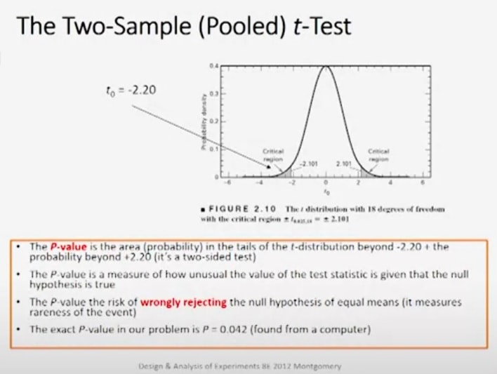
We saw that the computed value of the two-sample t-test statistic was minus 2.20 and that fell into the lower critical region of our t-distribution with 18 degrees of freedom. Now that was a fixed significance level test because that shows five percent to generate those critical values of 2.101 and minus 2.101, but the p-value is the probability or area in the tails beyond 2.20 and above plus 2.20 because it's a two-sided test. The p-value can be found in most cases by computers. |
It is the risk of wrongly rejecting the null hypothesis of equal means,in other words, it measures how unusual the event is.
The exact p-value in our problem turns out to be 0.042 and I've found that from a computer program, but you can approximate the p-value with a t-table.
Most t-tables only give probabilities greater than positive values of t. So just like we had to do with the normal distribution z-statistic,
take the absolute value of t0,which is minus 2.20, and turn it into a positive 2.20. Now with the value of 18 degrees of freedom, go into the t-table and see if you can find an exact value of 2.20. Well, you can't, but you can find values that bracket that.
2.101 is less than2.20 and 2.552 is greater than 2.20. So you can bracket this value quite nicely. The right tail probability for the smaller value 2.101 is 0.025 and for the larger value 2.552 is 0.01. Now you have to double those because this is a two-sided test.
So the p-value has to lie between 0.05 and 0.02. Those are lower and upper bounds on the p-value, and we know that the actual p-value turns out to be 0.042.
We find that from a computer program. Here is some two-sample t-test results
from computer software. The upper part of this tableis the output from a product called Minitab,which is a very nice,
very useful product for analyzing data. It's a good statistics package and the output we're seeing there is the two-sample t-test
for the Portland cement data. If you look through that output, you will find the estimated difference and you will find the value of the t-statistic minus 2.19.Now I got minus 2.20. The computer carried a few more decimal places than I
did and it has 18 degrees of freedom and the p-value is 0.042. At the bottom of the output table is the output from jump and once again, the calculation is very similar. The t-ratio is 2.186.
Notice it's positive instead of negative because the software subtracted them in a different order than I did, and then it gives you the standard error of the difference, that's the bottom of the t-ratio, 18 degrees of freedom, and here is the probability that the computed value is
greater than the absolute value of t,it's 0.0422, that is the two-sided p-value for this problem.So this is what computer output looks like and you're going to get some guidance onhow to actually use the software to obtain these numbers in another class. Checking assumptions in the t-test.
Now remember we're assuming that the observations come from a normal distribution and we
have also assumed that the variance of those normal distributions is the same. So we have two normal distributions with equal variances,
but possibly unequal means. How do we check those assumptions? Well, an easy way,
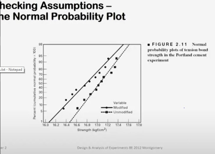
a convenient way to do that is with normal probability plotting. Here is a normal probability plot of the tension bond strength data from both samples of our Portland cement experiment. The solid dots are the modified mortar and the little rectangular plotting positions, those are the unmodified mortar.
Now when you look at this normal probability plot, the first thing I think that I see is that both of these samples tend to lie along straight lines and remember, in a normal probability plot, if the sample data does lie approximately along a straight line,that's some reasonable evidence that the samples are drawn from a normal distribution. So normality seems to be reasonable here.
It turns out that on the normal probability plot, the slope of the straight line is proportional to standard deviation.
So if the straight lines have similar or nearly identical slopes, then you feel pretty good about the assumption of constant variance. When I look at these plots, these lines, it looks to me like the slope of these two lines is very, very similar. Now if you're drawing these plots and interpreting them by hand, I always urge people to concentrate on the central portion of the plots when you visualize the straight line. Don't get too carried away with the tails because the bulk of the probability is in the center of the plot and that's what you want to use in deciding where to draw the straight line. How important are these assumptions? Well, the normality assumption is only moderately important. The t-test works pretty well even for moderate departures from normality. As long as the population is reasonably symmetric and reasonably unimodal, you're not going to have any real problems with the t-test. It's pretty robust to the normality assumption.
The constant variance assumption is more important. If you inadvertently make a wrong assumption there, it tends to impact the sensitivity of the test.
Its ability to detect differences is negatively impacted by that. So that's a more important assumption.
The exact p-value in our problem turns out to be 0.042 and I've found that from a computer program, but you can approximate the p-value with a t-table.
Most t-tables only give probabilities greater than positive values of t. So just like we had to do with the normal distribution z-statistic,
take the absolute value of t0,which is minus 2.20, and turn it into a positive 2.20. Now with the value of 18 degrees of freedom, go into the t-table and see if you can find an exact value of 2.20. Well, you can't, but you can find values that bracket that.
2.101 is less than2.20 and 2.552 is greater than 2.20. So you can bracket this value quite nicely. The right tail probability for the smaller value 2.101 is 0.025 and for the larger value 2.552 is 0.01. Now you have to double those because this is a two-sided test.
So the p-value has to lie between 0.05 and 0.02. Those are lower and upper bounds on the p-value, and we know that the actual p-value turns out to be 0.042.
We find that from a computer program. Here is some two-sample t-test results
from computer software. The upper part of this tableis the output from a product called Minitab,which is a very nice,
very useful product for analyzing data. It's a good statistics package and the output we're seeing there is the two-sample t-test
for the Portland cement data. If you look through that output, you will find the estimated difference and you will find the value of the t-statistic minus 2.19.Now I got minus 2.20. The computer carried a few more decimal places than I
did and it has 18 degrees of freedom and the p-value is 0.042. At the bottom of the output table is the output from jump and once again, the calculation is very similar. The t-ratio is 2.186.
Notice it's positive instead of negative because the software subtracted them in a different order than I did, and then it gives you the standard error of the difference, that's the bottom of the t-ratio, 18 degrees of freedom, and here is the probability that the computed value is
greater than the absolute value of t,it's 0.0422, that is the two-sided p-value for this problem.So this is what computer output looks like and you're going to get some guidance onhow to actually use the software to obtain these numbers in another class. Checking assumptions in the t-test.
Now remember we're assuming that the observations come from a normal distribution and we
have also assumed that the variance of those normal distributions is the same. So we have two normal distributions with equal variances,
but possibly unequal means. How do we check those assumptions? Well, an easy way,
a convenient way to do that is with normal probability plotting. Here is a normal probability plot of the tension bond strength data from both samples of our Portland cement experiment. The solid dots are the modified mortar and the little rectangular plotting positions, those are the unmodified mortar.
Now when you look at this normal probability plot, the first thing I think that I see is that both of these samples tend to lie along straight lines and remember, in a normal probability plot, if the sample data does lie approximately along a straight line,that's some reasonable evidence that the samples are drawn from a normal distribution. So normality seems to be reasonable here.
It turns out that on the normal probability plot, the slope of the straight line is proportional to standard deviation.
So if the straight lines have similar or nearly identical slopes, then you feel pretty good about the assumption of constant variance. When I look at these plots, these lines, it looks to me like the slope of these two lines is very, very similar. Now if you're drawing these plots and interpreting them by hand, I always urge people to concentrate on the central portion of the plots when you visualize the straight line. Don't get too carried away with the tails because the bulk of the probability is in the center of the plot and that's what you want to use in deciding where to draw the straight line. How important are these assumptions? Well, the normality assumption is only moderately important. The t-test works pretty well even for moderate departures from normality. As long as the population is reasonably symmetric and reasonably unimodal, you're not going to have any real problems with the t-test. It's pretty robust to the normality assumption.
The constant variance assumption is more important. If you inadvertently make a wrong assumption there, it tends to impact the sensitivity of the test.
Its ability to detect differences is negatively impacted by that. So that's a more important assumption.
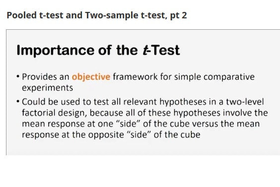
How important are these assumptions?
|
Why is the t-test an important procedure?
Well, I think that its biggest value is that
|
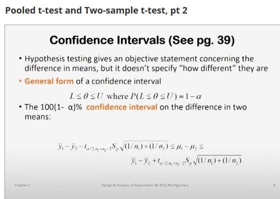
|
So that's the confidence interval and the confidence intervals will appear in this course again from time to time as useful ways to interpret data from designed experiments. |
A confidence interval is typically a statement of the form that you see here.
The parameters Theta and L and U are called the lower and upper confidence limits.
These limits are probability limits that are chosen in such a way so that the probability that Theta lies between L and U is equal to 1 minus Alpha.
The 100 times 1 minus Alpha percent confidence interval on the difference in two means, assuming of course that we have identical variances, is given by the equation at the bottom of the slide.
You'll notice that S sub p is used for the standard deviation. Then these are the lower and upper Alpha over 2 percentage points of the t-distribution with n1 plus n2 minus 2 degrees of freedom. We can actually calculate these intervals pretty easily for the Portland cement mortar formulation problem. We know everything, we know the two-sample averages, we know S square sub p, and we know that the appropriate t-percentile, the appropriate two and a half percentile point of t with 18 degrees of freedom is 2.101. So plugging those numbers into our confidence interval equation gives us a 95 percent confidence interval on the difference in means for minus 0.55, that's the lower bound, up to minus 0.01. Another way to say that is the confidence interval is minus 0.28 plus or minus 0.27 or the difference
in means strands for the accuracy of this interval is plus or minus 0.27. Notice, in looking at this interval, that zero is not in the interval. That's because we rejected the null hypothesis of equal means at the five percent level and this is a 95 percent confidence interval. If we had been unable to reject that null hypothesis at the five percent level, this interval would have included zero. So looking at a confidence interval, isn't the since another way to look at a hypothesis test? If the null hypothesis is not rejected, then the confidence interval on that parameter will include zero. So this is an alternate way to look at the results of the experiment and bet little bit more information. By the way, if you look at the computer output that we had earlier, both of these computer packages report a confidence interval. Minitab reports the confidence interval here and jump reports the confidence interval here. The signs are different on the lower and upper bound between these two computer outputs. Why is that? Well, that's because Jump did the calculations by subtracting the difference in means in a different order than Minitab did.
3 Classifications of statistics
|
1. Descriptive statistics
-organize and summarize date -NO attempt to generalize beyond sample -uses measure of central tendency and dispersion to describe characteristics of data -uses graphs to visually examine data characteristics What is central tendency? the mean, median, and mode What is the mean? average; sum of values divided by total number What is the median? -value where half fall above and half fall below; if number values are even, then the median is halfway bt the two middle values -arrange numbers from lowest to highest What is the mode? the most frequently occurring category (number) What are measures of dispersion? -range -variance -standard deviation What is the range? -diff bt highest and lowest value; subtract lowest number from the highest number -a wider range = a wider curve **What is variance? -measures the average deviation of values around a mean -reflects the range What is the standard deviation? -the square root of variance -average of how far each value in a group of values differs from the mean What is the most commonly used measure of dispersion in oral hygiene research? standard deviation What are the values in a normal distribution (normal curve)? -68% of values fall w/i 1 standard deviation of the mean -95% of values fall w/i 2 standard deviations of the mean -99.7% of values fall w/i 3 standard deviations of the mean All data analysis starts with descriptive statistics |
2. Inferential statistics
-allows us to infer or generalize conclusions from our sample back to original population -analyze data from sample to draw conclusions -sample data always differs slightly from population due to chance -quantifies (puts into #s) the degree of imprecision related to chance Statistical methods are based on? type and distribution of data What are parametric statistics? -interval and ratio data -normal distribution -large sample -ex: t test or anova What are non-parametric statistics? -less powerful bc has less info -nominal and ordinal -skewed distribution; will have + or - skew What does it mean to formulate a hypothesis? created a theory regarding the relationship bt independent and dependent variables A hypothesis will be broken down into? -null hypothesis (Ho): rejection of research;shows no relationship bt indep and dep variables -alternative hypothesis (H1): a way to explain phenomenon; there is a relationship bt the two variables Hypothesis errors with the null -type 1 error: reject null hypothesis when it is actually true; false positive -type 2 error: accept the null hypothesis when it is actually false; research showed was true, but is actually false-false negative It is easier to disprove the _________ hypothesis than to prove the __________ hypothesis null, alternative Testing the hypothesis -with a null hypothesis; often the reverse of what the experimenter actually believes -null put forward to allow the data to contradict it -trying to disprove null to show alternative hypothesis can be accepted alpha level is set before? statistical analysis What is alpha level? the amount of risk the researcher is willing to take related to committing a type 1 error; the probability of making a type 1 error Which type of error is worse case scenario? type 1; rejecting the null when it is actually true-false positive Alpha levels -.10 (10%) -.05 (5%) -.01 (1%) -choses before statistical analysis Which alpha level is the most common? -.05 (5%) -1/20 chance null will be rejected A type 2 error is related to a? beta level, usually .20 -20% chance of saying there is no relationship bt variable when there really is one What does statistical significance mean? probability that the observed diff arising by chance was sufficiently small If results are statistically significant, we can be confident that? our result happened bc of the independent variable and not by chance; we can reject the null hypothesis Level of significance is determined by a? p-value P-value is the chance of? -making a type 1 error; indicates how extreme data are P-value is related to? alpha level; if the p-value is less than alpha, the researcher can reject the null hypothesis If p-value is < alpha, then that equals? statistical significance |
3. Correlational statistics
-determines strength of relationship bt two variables -will show probable cause and effect -will be a direct or indirect correlation Correlational statistics produce what? correlation coefficient "r" (Pearson's r); a numerical value used to show how much two variables are related Correlation uses? -scatter plots to see relationship visually; will be + or - -parametric and non-parametric formulas Correlation will show? probably cause and effect, only strength and direction of relationship Pearson's r -parametric -r ranges from -1 to +1 -positive= one variable increases, other increases; direct relationship -negative= one variable increases, other decreases What does 0 correlation mean? no relationship bt variables; dots everywhere on scatter plot The closer the coefficient is to a value of -1 or +1, then? the stronger the relationship; can never achieve a perfect correlation of -1 or +1 With scatter plots, closer related variables make a __________ line indicating? straight, strong relationship Positive correlation -one variable increases, other increases -perfect positive +1 would be a straight line Negative correlation -one variable increases, other decreases -perfect negative -1 correlation would be straight line Chi square (X2) -non-parametric -used to determine if what is measured is statistically diff from what is expected (single sample) What does a chi square test? -the relationship bt CATEGORICAL variables -2 or more samples is nominal data -ex: is there a relationship bt gender and smoking -variable 1: gender (M/F) -variable 2: smoking (yes/no) What does an ANOVA do? -parametric -compares mean differences bt 2 OR MORE groups or 2 OR MORE variables -3 groups or more = ANOVA What does ANOVA stand for? ANalysis Of VAriance |
* Since the 1950's Numerous Cardiac Studies were done on Blood Group Tye A
* A and B RBC antigens fully develop 2 to 4 years of age
TERMS |
TERMS |
TERMS |
|
What does a t-test do?
-parametric -compares mean differences bt 2 diff samples OR 2 diff variables -treatment group and a control group The t-test is also called? Student's t-test A t-test will always only compare 2 groups What is a variable? anything that is being observed or measured; can be independent or dependent (a.k.a. Data) -ex: age, height, eye color, life expectancy, response toRx, teeth ... What is an independent variable? the intervention; what is being manipulated/changed What is the dependent variable? the outcome of interest; should change in response to the intervention "Plaque scores will < with > toothbrushing" What are the independent and dependent variables? -independent: increased toothbrushing -dependent: plaque scores what is an extraneous variable? unavoidable things that will effect the outcome of a study What type of study creates less chance of extraneous variables? larger and longer studies Distribution refers to? the spread of data/scores Natural variation of many variables follows a bell shaped curve; can be normal or skewed A skewed curve can be positive or negative; positive has long tail on (+) side, negative has long tail on (-) side With a normal bell shaped curve, the mean, median, and mode will? all be equal |
What do statistics do?
-analyze and interpret data of samples and populations -help determine how much of an observed changed occurred as a result of something or just by chance -tells us how much a change matters What is a parameter? population characteristic What is a statistic? numerical value that represents a sample characteristic What is categorical data? -limited set of values; only whole number, no averaging -ex: gender, number of DMFT, 1 or 2 kids (cannot be 1.3 kids) What is continuous data? -takes any value within a defined range -ex: bp, height, weight, time, age Categorical data is broken down into? nominal scales or ordinal scales Nominal scales -named categories -no mathematical relationship -ex: gender, eye color, yes/no answer Ordinal scales -ranks items in order; high to low, low to high -no mathematical relationship; no indication of how much higher/lower one item is in relation to another -ex: pain scale, stages of cancer Continuous data is broken down into? interval scales and ratio scales Interval scales -equal intervals bt data -NO true 0 point to indicate absence of something -ex: temperature; can never be an absence of temperature Ratio scales -interval bt values are consistent and meaningful -TRUE 0 point; complete absence of what is being measured ex: height, weight, bp |
Statistical model
A family of distributions dependent on a parameter t Parameter space The range of possible values for a parameter Estimator A function t^^ of data X_1,...,X_n with X_i ~ P_t such that t^^ is close to t Hypothesis test A function P ->{0.1} of data X_1,...,X_n with X_i ~ P_t such that P=0 with high probability if t = t_0 is close to t Confidence set A region which is a function C_n of data X_1,...,X_n with X_i ~ P_t such that P(t in C_n) = 1-a, for a in (0,1) fixed Likelihood The probability of occurrence of the observed sample given t Log-likelihood The logarithm of the likelihood function Normalised log-likelihood The logarithm of the likelihood function divided by the number of samples MLE An estimator t^^ which maximises the likelihood function given some data Score function The derivative of the log-likelihood Kullbach-Leibler distance The expectation of log(f(X;t_0)) - log(f(X;t)) over P_t_0 Regular A model in which integration wrt x and differentiation wrt t can be freely interchanged Fisher Information The variance of the score function Asymptotic efficiency n Var_t (t^^) -> I(t)^-1 as n -> infinity Consistent An estimator which converges in probability to the true value of t as n -> infinity Almost surely Convergence st P(||X_n - X|| -> 0 as n -> infinity) = 1 In Probablility Convergence st P(||X_n - X|| < e) -> 0 for all e>0, as n -> infinity In distribution Convergence st P(X_n < t) -> P(X < t) as n -> infinity, wherever P(X < t) is continuous in t Observed Fisher information The normalised sum of the derivative of the log-likelihood times its transpose Wald statistics The statistics W_n(t) = n(t^^ - t_0)^T i^^_n (t^^ - t_0) Type I error Rejecting the null hypothesis when it is true Type II error Accepting the null hypothesis when it is false Score test Using the statistic 1/sqrt(n) d/dt l_n(t) which converges to N(0,I^-1(t_0)) in distribution, to test a simple null hypothesis |
Jeffrey's prior
A prior distribution proportional to the square root of the determinant of the fisher information Action space The set of possible actions for a decision rule Decision rule A function from the state space to the action space Risk R(d,t_0) = E_(t_0) [L(d(X),t_0)] Bayes risk R_pi(d) = E_pi[R(d,t)] Posterior risk The expected loss over the posterior distribution Minimax A decision rule which attains the least maximum risk Least favourable A prior whose Bayes' rule has greater Bayes risk than any other prior Inadmissible A decision rule with an alternative rule whose risk is no more than the original rule, and strictly less at some points of t Admissible Not inadmissible Risk set The possible values of the risk given t fixed, over all decision rules James-Stein estimator The estimator for the mean of a normal model of dimension at least 3 given by (1-(p-2)/||X||^2)X Covariance Of real-valued random variables X and Y: E((X-E[X])(Y-E[Y])) Correlation Of real-valued random variables X and Y: the covariance divided by the square root of the product of their individual variances Jacknife bias estimate (n-1)(Sum(T_(-i))/n - T_n)) for a biased estimator T_n Importance sampling To approximate the mean of g(X), where X ~ f, we sample Z with density h and use g(Z)f(Z)/h(Z) Accept/reject An algorithm to simulate Y ~ f, by generating X ~ h where f <= Mh, and generate U ~ U([0,1]), and accepting X if U < f(X)/Mh(X), if not try again. Empirical distribution F_n(x) = 1/n Sum(indicator{x >= X_i}) given observations X_1,...,X_n Cramer-Rao [Theorem] The variance of an estimator T' of T is at least (d/dT E_T(T'))^2/n I(T), where I is the Fisher information. Continuous mapping [Theorem] If g:S->R is continuous, X_n->X by some manner, then also g(X_n)->g(X), by the same manner. Slutsky [Theorem] If X_n->X, Y_n->c in distribution, then Y_n->c in probability, X_n+Y_n->X+c in distribution, X_n Y_n -> cX in distribution, and if c =/=0, X_n/Y_n -> X/c in distribution WLLN The mean of n observations converges in probability to the expectation SLLN The mean of n observations converges almost surely to the expectation Central Limit [Theorem] sqrt(n) (mean - expectation) -> N(0,Var(X)) Wilks [Theorem] If H_0 has dimension d_0, H_1 dimension d, then the likelihood ratio statistic converges to a chi^2 on d-d_0 Bernstein von Mises [Theorem] If pi is a continuous prior, pi_n the posterior, and P_n ~ N(T_MLE, I(T)^-1/n), then the integral of |pi_n - P_n| -> 0 almost surely as n-> infinity Stein [Theorem] If X ~ N(T,1), g differentiable, bounded, E_T(g'(X))=E_T(g(X)(X-T)) when finite Gliverto-Cantelli [Theorem] The empirical distribution converges uniformly almost surely to the real distribution Kolmogorov-Smirnov [Theorem] sqrt(n)||F_n-F|| -> ||B|| in distribution for a standard Brownian bridge B, F_n an empirical distribution. |
